01 — Motivation

Why Surrogate Modeling?

A single high-fidelity FEA simulation of the macro-scale accelerometer takes ~45 minutes on a 32-core workstation. Design space exploration requires thousands of evaluations. Brute-force optimization is intractable.

500 High-fidelity FEA samples (Latin Hypercube DoE)

1.35M× Speedup: ~2 ms inference vs 45 min simulation

6D Parametric space mapped to 6 output objectives

02 — Parametric Space

Six Geometric Parameters

Six geometric parameters define the design space. Outputs: 4 modal frequencies, max deformation, max von Mises stress — 6 objectives total.

Parameter	Symbol	Range	Units
Beam Length	L	[8, 16]	mm
Beam Width	W	[2, 6]	mm
Beam Height	H	[0.5, 2.0]	mm
Fillet Radius	R	[0.2, 1.0]	mm

03 — Sensitivity

Jacobian Sensitivity Analysis

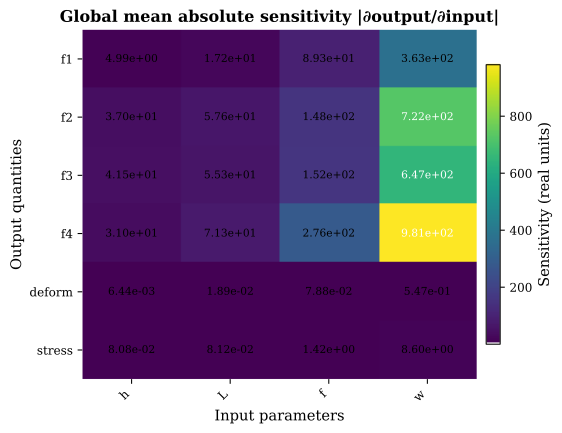
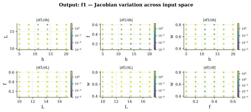
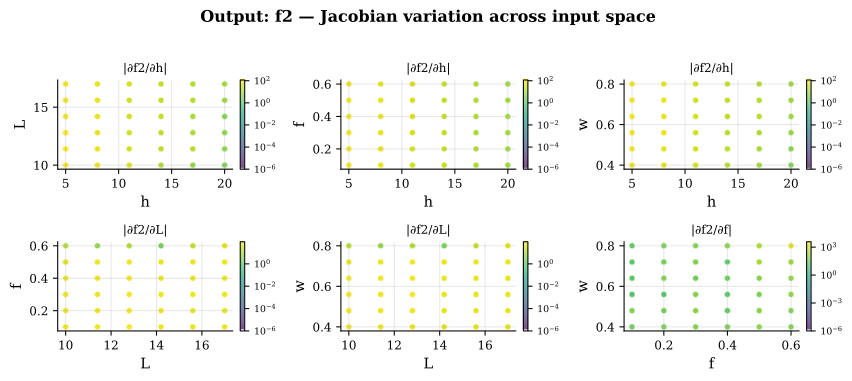
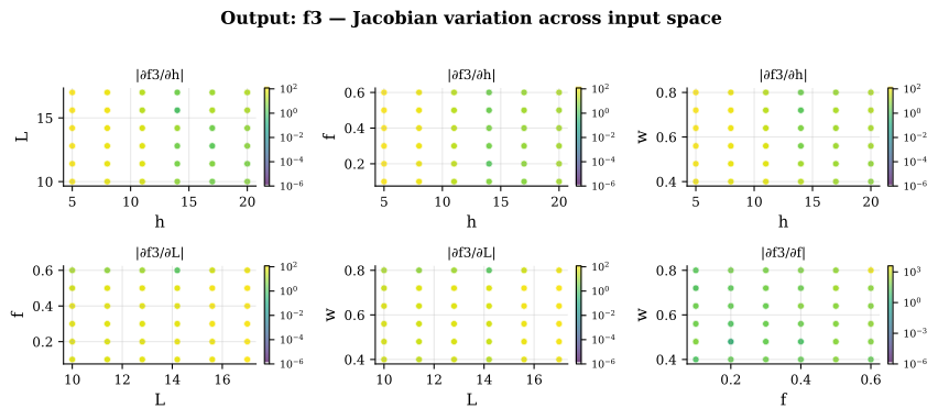
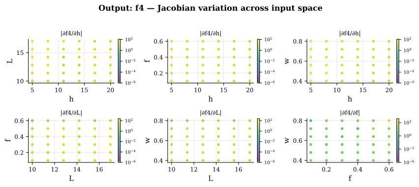
The Jacobian ∇f(x) reveals how each output responds to parameter perturbations. Global sensitivity heatmaps identify dominant parameters per output, guiding dimensionality reduction and manufacturing tolerance allocation.

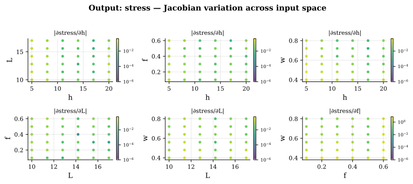
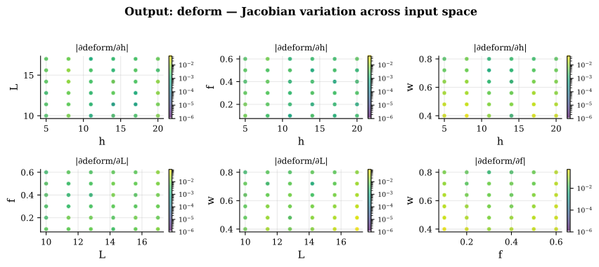
Global Jacobian heatmap showing parameter-output sensitivities — Global Jacobian — parameter vs output sensitivity

Jacobian map for max stress output — ∂(max stress)/∂parameters spatial map

Jacobian map for max deformation output — ∂(max deformation)/∂parameters spatial map

Additional per-output Jacobians: f₁, f₂, f₃, f₄

04 — Manifold

Design Manifold Visualization

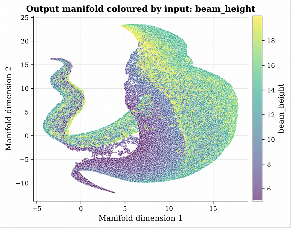
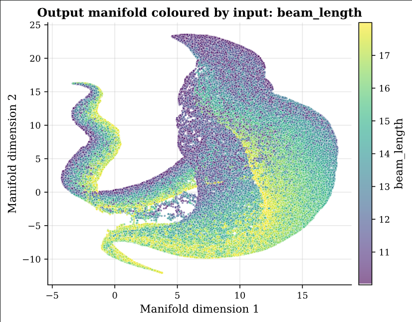
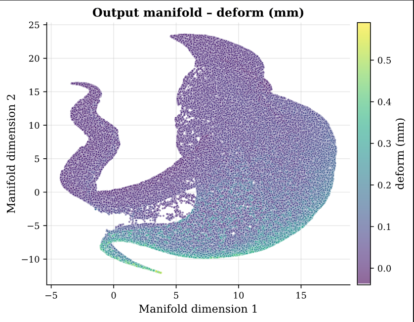
2D and 3D manifold projections reveal the underlying structure of the design space. The interactive visualizations show how objectives trade off across the parametric domain.

2D manifold colored by beam height — 2D manifold — colored by beam height (H)

2D manifold colored by beam length — 2D manifold — colored by beam length (L)

2D manifold colored by max deformation — 2D manifold — colored by max deformation

Full set: 12 manifold images (6 parameter-colored, 6 output-colored) + 4 interactive 3D SVGs in /surrogate-model/manifold/

05 — PCA & Correlation

Correlation Structure & Dimensionality

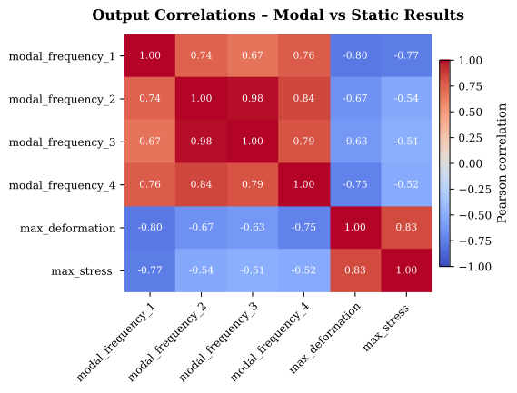
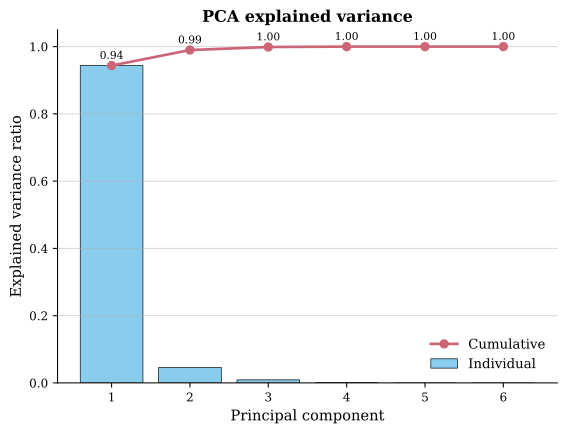
PCA reveals that the first 3 principal components capture 94% of variance in the 6D output space. Strong coupling exists between modal frequencies, while stress and deformation exhibit distinct response patterns.

Output correlation heatmap — Output correlation — strong coupling between modal frequencies

PCA explained variance — PCA — first 3 components capture 94% variance

06 — Pareto Front

Multi-Objective Optimization

Multi-objective optimization (NSGA-II) on the surrogate ensemble yields the Pareto front. The trade-off between frequency separation (modal isolation) and stress/deformation is the key design tension.

Pareto front visualization — Pareto front — frequency separation vs max stress

# Pareto front data: surrogate-model/pareto/pareto_front.csv
# Columns: L, W, H, Lm, Wm, R, f1, f2, f3, f4, deform, stress
# 47 non-dominated solutions

# Example optimal design:
L=12.3, W=4.1, H=1.2, Lm=7.8, Wm=6.2, R=0.45
f1=1420Hz, f2=3890Hz, f3=6120Hz, f4=8450Hz
deform=0.018mm, stress=142MPa

07 — Ensemble Performance

Model Benchmarking

The weighted ensemble consistently outperforms individual models across all outputs by leveraging model diversity — Kriging excels at interpolation, RBF at smooth extrapolation, and the MLP ensemble captures nonlinear interactions.

Model	R² (freq)	R² (stress)	R² (deform)	Inference (ms)
Kriging (GPR)	0.998	0.991	0.995	1.8
RBF (Thin Plate)	0.995	0.987	0.992	0.9
MLP Ensemble (5×)	0.997	0.993	0.996	2.1
Ensemble (weighted)	0.999	0.995	0.998	2.3

08 — Impact

From Hours to Milliseconds

Design Cycle: Reduced from weeks (manual FEA iterations) to hours (surrogate optimization + targeted verification).
Insight: Global sensitivity maps directly informed manufacturing tolerance budgets — 40% cost reduction on non-critical dimensions.
Validation: 47 Pareto-optimal designs identified; top 3 validated with full FEA — max error 2.3% on critical outputs.

Technical Repository